Using XGBoost with Tidymodels
Andy Merlino and Nick Merlino
2020/05/19

Background
XGBoost is a machine learning library originally written in C++ and ported to R in the xgboost R package. Over the last several years, XGBoost’s effectiveness in Kaggle competitions catapulted it in popularity. At Tychobra, XGBoost is our go-to machine learning library.
François Chollet and JJ Allaire summarize the value of XGBoost in the intro to “Deep Learning in R”:
In 2016 and 2017, Kaggle was dominated by two approaches: gradient boosting machines and deep learning. Specifically, gradient boosting is used for problems where structured data is available, whereas deep learning is used for perceptual problems such as image classification. Practitioners of the former almost always use the excellent XGBoost library.
These are the two techniques you should be the most familiar with in order to be successful in applied machine learning today: gradient boosting machines, for shallow-learning problems; and deep learning, for perceptual problems. In technical terms, this means you’ll need to be familiar with XGBoost and Keras—the two libraries that currently dominate Kaggle competitions.
At Tychobra, we have trained XGBoost models using the caret R package created by Max Kuhn. caret has treated us very well over the years (check out our post Machine Learning for Insurance Claims for an example of using xgboost with caret).
Max Kuhn and others at Rstudio have more recently turned their attention from caret to “tidymodels” (the successor to caret). “tidymodels” is a collection of R packages that work together to simplify and supercharge model training and tuning. With the recent launch of tidymodels.org, we felt it was time to give the tidymodels R packages a shot.
Overview
In this post we will train and tune an XGBoost model using the tidymodels R packages. We use the AmesHousing dataset which contains housing data from Ames, Iowa. Our model will predict house sale price.
# data
library(AmesHousing)

# data cleaning
library(janitor)

# data prep
library(dplyr)

# tidymodels
library(rsample)
library(recipes)
library(parsnip)
library(tune)
library(dials)
library(workflows)
library(yardstick)

# speed up computation with parrallel processing (optional)
library(doParallel)
all_cores <- parallel::detectCores(logical = FALSE)
registerDoParallel(cores = all_cores)
Load in the Ames housing dataset.
# set the random seed so we can reproduce any simulated results.
set.seed(1234)

# load the housing data and clean names
ames_data <- make_ames() %>%
  janitor::clean_names()
Step 0: EDA (Exploratory Data Analaysis)
At this point we would normally make a few simple plots and summaries of the data to get a high-level understanding of the data. For simplicity, we are going to cut the EDA process from this post, but, in a real-world analysis, understanding the business problems and doing effective EDA are often the most time consuming and crucial aspects of the analysis.
Step 1: Initial Data Split
Now we split the data into training and test data. Training data is used for the model training and hyperparameter tuning. Once trained, the model can be evaluated against test data to assess accuracy.
# split into training and testing datasets. Stratify by Sale price
ames_split <- rsample::initial_split(
  ames_data,
  prop = 0.8,
  strata = sale_price
)
Step 2: Preprocessing
Preprocessing alters the data to make our model more predictive and the training process less compute intensive. Many models require careful and extensive variable preprocessing to produce accurate predictions. XGBoost, however, is robust against highly skewed and/or correlated data, so the amount of preprocessing required with XGBoost is minimal. Nevertheless, we can still benefit from some preprocessing.
In tidymodels, we use the recipes package to define these preprocessing steps, in what is called a “recipe”.
# preprocessing "recipe"
preprocessing_recipe <-
  recipes::recipe(sale_price ~ ., data = training(ames_split)) %>%
  # convert categorical variables to factors
  recipes::step_string2factor(all_nominal()) %>%
  # combine low frequency factor levels
  recipes::step_other(all_nominal(), threshold = 0.01) %>%
  # remove no variance predictors which provide no predictive information
  recipes::step_nzv(all_nominal()) %>%
  prep()
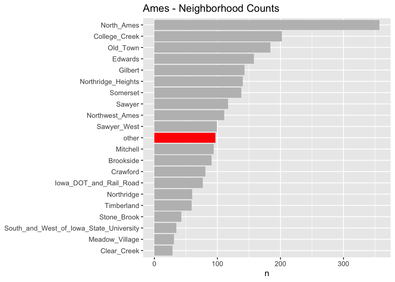
As you can see in the chart below, for the “neighborhood” variable, several of the factor levels with the fewest observations (less than 1% of the total number of observations) have been lumped into an “other” factor level. We did this preprocessing in step_other() in the above recipe.

Step 3: Splitting for Cross Validation
We apply our previously defined preprocessing recipe with bake(). Then we use cross-validation to randomly split the training data into further training and test sets. We will use these additional cross validation folds to tune our hyperparameters in a later step.
ames_cv_folds <-
  recipes::bake(
    preprocessing_recipe,
    new_data = training(ames_split)
  ) %>%
  rsample::vfold_cv(v = 5)
Step 4: XGBoost Model Specification
We use the parsnip package to define the XGBoost model specification. Below we use boost_tree() along with tune() to define the hyperparameters to undergo tuning in a subsequent step.
# XGBoost model specification
xgboost_model <-
  parsnip::boost_tree(
    mode = "regression",
    trees = 1000,
    min_n = tune(),
    tree_depth = tune(),
    learn_rate = tune(),
    loss_reduction = tune()
  ) %>%
    set_engine("xgboost", objective = "reg:squarederror")
Step 5: Grid Specification
We use the tidymodel dials package to specify the parameter set.
# grid specification
xgboost_params <-
  dials::parameters(
    min_n(),
    tree_depth(),
    learn_rate(),
    loss_reduction()
  )
Next we set up the grid space. The dails::grid_* functions support several methods for defining the grid space. We are using the dails::grid_max_entropy() function which covers the hyperparameter space such that any portion of the space has an observed combination that is not too far from it.
xgboost_grid <-
  dials::grid_max_entropy(
    xgboost_params,
    size = 60
  )

knitr::kable(head(xgboost_grid))| min_n | tree_depth | learn_rate | loss_reduction |
|---|---|---|---|
| 34 | 1 | 0.0118682 | 29.9649253 |
| 38 | 12 | 0.0001291 | 0.6156496 |
| 6 | 7 | 0.0000949 | 0.0000000 |
| 32 | 4 | 0.0000005 | 0.0000367 |
| 14 | 2 | 0.0001833 | 0.0000000 |
| 31 | 8 | 0.0000000 | 1.4345098 |
To tune our model, we perform grid search over our xgboost_grid’s grid space to identify the hyperparameter values that have the lowest prediction error.
Step 6: Define the Workflow
We use the new tidymodel workflows package to add a formula to our XGBoost model specification.
xgboost_wf <-
  workflows::workflow() %>%
  add_model(xgboost_model) %>%
  add_formula(sale_price ~ .)
Step 7: Tune the Model
Tuning is where the tidymodels ecosystem of packages really comes together. Here is a quick breakdown of the objects passed to the first 4 arguments of our call to tune_grid() below:
- “object”: xgboost_wf which is a workflow that we defined by the parsnip and workflows packages
- “resamples”: ames_cv_folds as defined by rsample and recipes packages
- “grid”: xgboost_grid our grid space as defined by the dials package
- “metric”: the yardstick package defines the metric set used to evaluate model performance
# hyperparameter tuning
xgboost_tuned <- tune::tune_grid(
  object = xgboost_wf,
  resamples = ames_cv_folds,
  grid = xgboost_grid,
  metrics = yardstick::metric_set(rmse, rsq, mae),
  control = tune::control_grid(verbose = TRUE)
)
In the above code block tune_grid() performed grid search over all our 60 grid parameter combinations defined in xgboost_grid and used 5 fold cross validation along with rmse (Root Mean Squared Error), rsq (R Squared), and mae (Mean Absolute Error) to measure prediction accuracy. So our tidymodels tuning just fit 60 X 5 = 300 XGBoost models each with 1,000 trees all in search of the optimal hyperparameters. Don’t try that on your TI-83!
These are the hyperparameter values which performed best at minimizing RMSE.
xgboost_tuned %>%
  tune::show_best(metric = "rmse") %>%
knitr::kable()| min_n | tree_depth | learn_rate | loss_reduction | .metric | .estimator | mean | n | std_err |
|---|---|---|---|---|---|---|---|---|
| 12 | 7 | 0.0346875 | 0.0451186 | rmse | standard | 25561.99 | 5 | 2983.927 |
| 9 | 13 | 0.0183617 | 0.1042750 | rmse | standard | 25576.99 | 5 | 2687.849 |
| 23 | 5 | 0.0788798 | 0.7513677 | rmse | standard | 25645.38 | 5 | 2461.057 |
| 11 | 6 | 0.0091690 | 0.0000001 | rmse | standard | 25669.84 | 5 | 2706.457 |
| 10 | 2 | 0.0108475 | 0.0000003 | rmse | standard | 25883.23 | 5 | 2828.172 |
Next, isolate the best performing hyperparameter values.
xgboost_best_params <- xgboost_tuned %>%
  tune::select_best("rmse")

knitr::kable(xgboost_best_params)| min_n | tree_depth | learn_rate | loss_reduction |
|---|---|---|---|
| 12 | 7 | 0.0346875 | 0.0451186 |
Finalize the XGBoost model to use the best tuning parameters.
xgboost_model_final <- xgboost_model %>%
  finalize_model(xgboost_best_params)
Step 8: Evaluate Performance on Test Data
Now that we have trained our model, we need to evaluate the model performance. We use test data from step 1 (data that was not used in the model training) to evaluate performance.
We use the rmse (Root Mean Squared Error), rsq (R Squared), and mae (Mean Absolute Value) metrics from the yardstick package in our model evaluation.
First let’s evaluate the metrics on the training data:
train_processed <- bake(preprocessing_recipe,  new_data = training(ames_split))

train_prediction <- xgboost_model_final %>%
  # fit the model on all the training data
  fit(
    formula = sale_price ~ .,
    data    = train_processed
  ) %>%
  # predict the sale prices for the training data
  predict(new_data = train_processed) %>%
  bind_cols(training(ames_split))

xgboost_score_train <-
  train_prediction %>%
  yardstick::metrics(sale_price, .pred) %>%
  mutate(.estimate = format(round(.estimate, 2), big.mark = ","))

knitr::kable(xgboost_score_train)| .metric | .estimator | .estimate |
|---|---|---|
| rmse | standard | 3,807.24 |
| rsq | standard | 1.00 |
| mae | standard | 2,747.17 |
And now for the test data:
test_processed  <- bake(preprocessing_recipe, new_data = testing(ames_split))

test_prediction <- xgboost_model_final %>%
  # fit the model on all the training data
  fit(
    formula = sale_price ~ .,
    data    = train_processed
  ) %>%
  # use the training model fit to predict the test data
  predict(new_data = test_processed) %>%
  bind_cols(testing(ames_split))

# measure the accuracy of our model using `yardstick`
xgboost_score <-
  test_prediction %>%
  yardstick::metrics(sale_price, .pred) %>%
  mutate(.estimate = format(round(.estimate, 2), big.mark = ","))

knitr::kable(xgboost_score)| .metric | .estimator | .estimate |
|---|---|---|
| rmse | standard | 30,217.58 |
| rsq | standard | 0.87 |
| mae | standard | 15,728.22 |
The above metrics on the test data are significantly worse than our training data metrics, so we know that there is some overfitting going on in our model. This highlights the importance of using test data, rather than training data, to evaluate model performance.
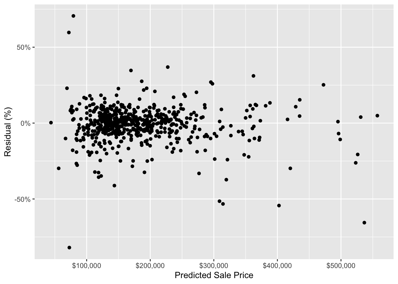
To quickly check that there is not an obvious issue with our model’s predictions, let’s plot the test data residuals.
house_prediction_residual <- test_prediction %>%
  arrange(.pred) %>%
  mutate(residual_pct = (sale_price - .pred) / .pred) %>%
  select(.pred, residual_pct)

ggplot(house_prediction_residual, aes(x = .pred, y = residual_pct)) +
  geom_point() +
  xlab("Predicted Sale Price") +
  ylab("Residual (%)") +
  scale_x_continuous(labels = scales::dollar_format()) +
  scale_y_continuous(labels = scales::percent)
The above chart does not show any super obvious trends in the residuals. This indicates that, at a very high level, our model is not systematically making inaccurate predictions for houses with certain predicted sale prices. We would do more model validation here for a real-world analysis, but, for the sake of this post, the above chart is good enough for us.
Conclusion
In this post, we were not overly concerned with our model’s performance. Our goal was to simply work through the process of training an XGBoost model using tidymodels, and to learn the tidymodels basics along the way.
Tidymodels gives us a standard process and vocabulary to handle resampling (rsample), data preprocessing (recipes), model specification (parsnip), tuning (tune), and model validation (yardstick). The work done by the tidymodels team to “tidy” the machine learning process is a step change improvement for approachability to machine learning in R; it is easier than ever to train and (more importantly) understand the model training process using the tidymodels packages. Thank you tidymodels team!
We are still just getting started with tidymodels, so please let me know if you see errors or have suggestions for improvements!
Similar Work
If you liked this post, you should check out this excellent post by Business Science which goes into a lot more detail in the EDA process and also trains a glmnet model.
comments powered by Disqus